In this post, I am going to demonstrate a two-step Scala implementation of Radial Basis Function Neural Network (RBFNetwork): (unsupervised) k-means clustering first, and (supervised) gradient descent second. This two-step implementation is fast and efficient compared to Multilayer Perceptron while providing good predictive performance. This is because unsupervised learning at the first step provides information about data distribution so that the second step can have an intuition about the data and fine-tune the model.
For us, most of the Machine Learning models that we use today are just black box approaches that we take from some library. It is good to have this ability for faster development; however, it would be nicer to know internal dynamics of their implementations. Therefore, I am hoping that this post will be simple enough to provide you that information.
Implementation
Let’s start with introducing the abstractions that we are going to use for the rest of the code.
Function Aliases
Since the most granular abstraction is a function, here below we are going to name them based on their actual job in this implementation:
type Features = IndexedSeq[Double]
type DistanceFunc = ((IndexedSeq[Double], IndexedSeq[Double]) => Double)
type RadialBasisFunction = (IndexedSeq[Double] => Double)
type Clustering = () => IndexedSeq[(Features, IndexedSeq[Features])]
This definition is useful since it lets us write more readable code. Remember: we write code for humans to understand, assuming that the computer somehow is going to understand it anyway. For example, you can read the above code like this:
Distance is a function that takes two points from n-dimensional space specified with IndexedSeq‘s size and produces an output metric of type double.
Let’s move forward with introducing higher-level abstractions like traits.
Traits
You can think of a trait as a recipe for doing something; however, it is not something by itself. It is preferable over abstract classes when you want to take advantage of mixing classes, but the end goal is the same: you want to have a resuable set of behaviors somewhere in your code that you can use anytime to add any class that conforms to the protocol that you declare within the trait. An example of this would be gradient descent. It can actually optimize a lot of Machine Learning algorithms, not just neural networks or something else. Therefore, we can think of it as a recipe for optimizing a neural network algorithm. Down below, we define this set of behaviors.
import Math.{exp,pow,sqrt}
import scala.annotation.tailrec
import scala.util.Random
trait Optimizer {
  def fit(dataSet: Iterable[(IndexedSeq[Double], IndexedSeq[Double])], learningRate: Double)
}
trait NeuralNetworkModel extends (IndexedSeq[Double] => IndexedSeq[Double]) {
  def getH(input: (IndexedSeq[Double], IndexedSeq[Double])):IndexedSeq[Double]
}
trait EuclideanDistance extends DistanceFunc {
  override def apply(position1: IndexedSeq[Double], position2: IndexedSeq[Double]): Double = {
    val sum = position1.zip(position2).map {
      case (p1, p2) =>
        val d = p1 - p2
        pow(d,2)
    }.sum
    sqrt(sum)
  }
}
trait GradientDescent extends Optimizer with NeuralNetworkModel {
  val nHidden: Int
  val weights: Array[Double]
  def fit(trainingData: Iterable[(IndexedSeq[Double], IndexedSeq[Double])], learningRate: Double = 0.1): Unit  = {
    for(pair <- trainingData){
      val actual = this(pair._1)
      val X = getH(pair)
      val desired = pair._2
      for( outputIndex <- desired.indices) {
        val error = desired(outputIndex) - actual(outputIndex)
        val update = X.indices.map(i => learningRate * X(i) * error)
        X.indices.foreach { i =>
          val weightIndex = (nHidden  * outputIndex) + i
          weights(weightIndex) = update(i) + weights(weightIndex)
        }
        //bias term
        val weightIndex = (nHidden  * outputIndex) + X.length
        weights(weightIndex) = learningRate * error + weights(weightIndex)
      }
    }
  }
}
We can even think of k-means as a trait and change its distance function that it uses for its internal clustering calculation according to the same convention. Down below, we move forward with this.
trait RadialBasisFunctionNetworkTrait extends NeuralNetworkModel {
  val nIn: Int
  val nOut: Int
  val rbfs: IndexedSeq[RadialBasisFunction]
  val nHidden: Int = rbfs.length + 1
  val weights: Array[Double] = Array.fill(nHidden * nOut)(scala.math.random)
  override def getH(input: (IndexedSeq[Double], IndexedSeq[Double])):IndexedSeq[Double] = {
    rbfs.indices.map { i => rbfs(i)(input._1) }
  }
  override def apply(input: IndexedSeq[Double]): IndexedSeq[Double] = {
    for (outputIndex <- 0 until nOut) yield {
      val linearCombination = rbfs.indices.map { i => rbfs(i)(input) * weights((nHidden * outputIndex) + i)}
      val bias = weights((nHidden * outputIndex) + rbfs.length)
      linearCombination.sum + bias
    }
  }
}
abstract class KMeans(val seed: Int, val k: Int, val eta: Double, val data: Vector[Features]) extends DistanceFunc with Clustering {
  val rand = new Random(seed)
  val _data = data
  val means: Vector[Features] = (0 until k).map(_ => data(rand.nextInt(data.length))).toVector
  def apply(): IndexedSeq[(Features, IndexedSeq[Features])] = {
    @tailrec
    def _kmeans(means: IndexedSeq[Features]): IndexedSeq[(Features, IndexedSeq[Features])] = {
      val newMeans: IndexedSeq[(Features, IndexedSeq[Features])] =
        means.map(mean => {
          _data.groupBy(p => means.minBy(m => this (m, p))).get(mean) match {
            case Some(c) => (c.transpose.map(_.sum).map(x => x / c.length), c)
            case _ => (mean, Vector(mean))
          }
        })
      val converged = (means zip newMeans.map(_._1)).forall {
        case (oldMean, newMean) => this (oldMean, newMean) <= eta
      }
      if (!converged) _kmeans(newMeans.map(_._1)) else newMeans
    }
    _kmeans(means)
  }
}
type ErrorFunc = (NeuralNetworkModel, Iterable[(IndexedSeq[Double], IndexedSeq[Double])]) => Double
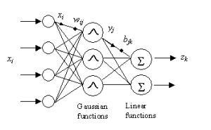
Let’s read above code like this: We have a NeuralNetworkModel that takes an input that consists of features like IndexedSeq and produces target values as again IndexedSeq, this is because neural networks may produce multi outputs like in the case of mutliclass classification. We define this behavior by extending Function[IndexedSeq[Double],IndexedSeq[Double]]. It also declares getH in its protocol, which means that any class that implements this needs to tell how to get hidden values from the pair of input and target values. In the case of RBFNetwork it applies a Gaussian Function to its inputs in its hidden layer. Therefore, when we call getH, RBFNetwork may want to return these values. Now, let’s create a K-means implementation that uses Euclidean Distance as a distance function and RBFNetwork with the Gradient Descent optimizer.
case class KMeansImpl(override val seed: Int,override val k: Int,override val eta: Double,override val data: Vector[Features]) extends KMeans(seed, k, eta , data)
        with EuclideanDistance
case class RadialBasisFunctionNetwork(nIn: Int, nOut: Int, rbfs: IndexedSeq[RadialBasisFunction])
     extends RadialBasisFunctionNetworkTrait
     with GradientDescent
That is it. Let’s analyze an example of the dataset using this code.
Inference
In this example, we have two by 50 training data and two by 100 validation data. The end goal is to construct a regression model. The first column is an input and the second column is a target or in the other words respondent variable. We are going to use Gaussian Function as a Radial Basis Function component for the neural network and use Gradient Descent as an optimizer. To initialize Gaussian Functions’ center and width, we are going to run the K-means algorithm and take means as a center for the Gaussian Function and the maximum distance between cluster elements and its mean as a width for the same function. We are going to run this pipeline with a different amount of Gaussian Experts in the other words with different hidden layer sizes and evaluate their performance so that we can observe one underfitting model, one overfitting model, and one good fit model.
def trainAndGetModel(rbfCount: Int, training:Vector[(Vector[Double], Vector[Double])]) = {
    val kmeansImpl = KMeansImpl(seed = 1990, k = rbfCount, eta = 1E-5, data = training.map(_._1))
    val clusters = kmeansImpl()
    val radialBasisFunctions = clusters.map { case (means, cluster) => GaussianFunction(width = cluster.map(it => kmeansImpl(it, means)).max, center = means) }
    val net = new RadialBasisFunctionNetwork(nIn = 1,rbfs = radialBasisFunctions,nOut = 1)
    for (i <- 0 to 500)
      net.fit(training,0.1)
    net
}
val models =
    (for{i <- 1 to 10} yield {
        ( i -> trainAndGetModel(rbfCount=i,trainingData))
    })
Visualization
Above, we trained 10 different models with 500 iterations with different hidden layer sizes (Gaussian unit counts) ranging from 1 to 10. We could have had different results by changing learningRate; in this case, it is 0.1 since it gave us the minimum RMSE error. Let’s look at these 10 models RMSE results on both the training dataset and the test dataset. Let’s look at RMSE on both training and test set respectively.
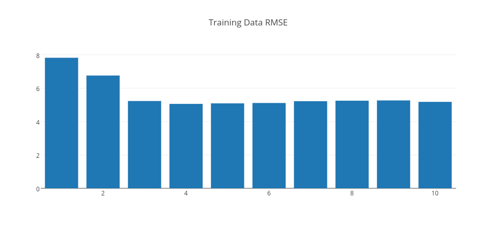
As is expected, the training RMSE is decreasing consistently as the Gaussian unit count increases. However, we need to look at test errors for choosing the right model.
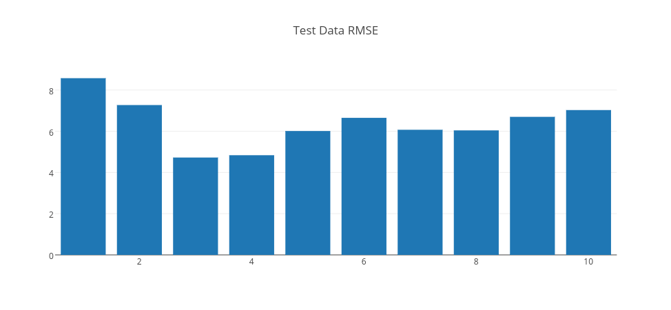
By analyzing RMSE errors on the graph, we can conclude that when RBF count is 1, it is seen that the error is high for both training and test data. So, this is an example of an underfit model. When RBF count is 3, the error drops significantly to the minimum on the test data. So, we can pick this model as a good fit model. However, when RBF count is higher than 3, the error gets higher on the test data. So, this is a sign that the model is overfitting, as the model gets more complex with more RBF units. Thus, a model with 10 RBF units is an example of overfitting model.
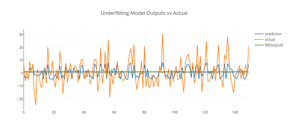
Let’s pick those models and see their predictions in conjunction with actual data and RBF outputs.
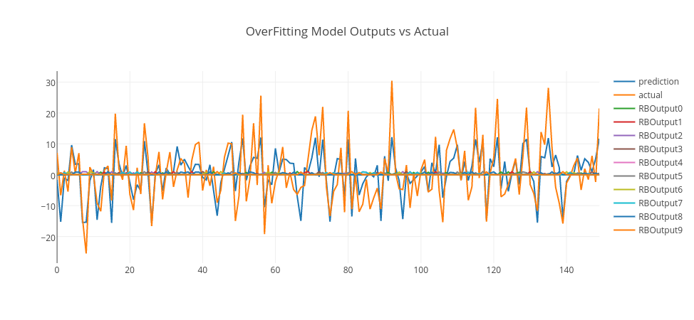
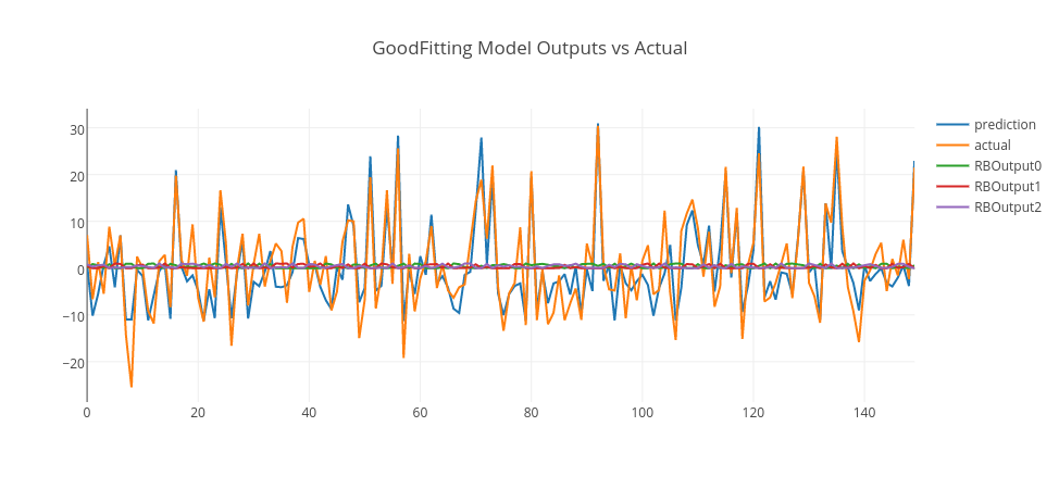
Conclusion
In the above graphs, we merged training and test data and plot model predictions, RBF outputs, and actual data. As it is clearly seen, the underfitting model produces an output close to random that goes around zero — it doesn’t even model the training data. The overfitting model is more responsive to the noise on the training data; however, it doesn’t generalize well. However, the good-fitting model is well on both training and test data. You can experiment this by yourself using this GitHub repo and enjoy.